Working with Data

Overview

Teaching: 20 min
Exercises: 10 min

Questions

How should I work with numeric data in Python?

What’s the recommended way to handle and analyse tabular data?

How can I import tabular data for analysis in Python and export the results?

Objectives

handle and summarise numeric data with NumPy.

filter values in their data based on a range of conditions.

load tabular data into a pandas dataframe object.

describe what is meant by the data type of an array/series, and the impact this has on how the data is handled.

add and remove columns from a dataframe.

select, aggregate, and visualise data in a dataframe.

Unlike languages like R and MATLAB, Python wasn’t designed with any specific purpose, such as statistical programming, in mind. This has some advantages, e.g. it’s generally easier to adapt Python to whatever task you want to perform, than it is to apply a more domain-specific language to the type of task for which it wasn’t designed in the first place. But it also has some disadvantages, e.g. as a Python user you have to take extra steps to begin working with and analysing data.

Python has no built-in datatypes intended for efficient computation on numeric or tabular data. You could create elaborate, nested structures combining lists, dictionaries, and sets, to produce something that allows you to handle and summarise a data table in the convenient way you want to. If you learn how to write your own classes (beyond the scope of this course) you could even encapsulate those complex data structures and re-use them elsewhere. But that’s a lot of effort to create something that would probably be very inefficient from a code performance perspective. And anyway, it’s not really the way you’re supposed to do things with Python. Instead, we can benefit from the hard work and expertise of others who have already taken on this challenge, creating whole libraries devoted to working with different kinds of data.

In this section, we’ll focus on two of the most well-known and widely-used examples: NumPy and pandas. Unlike everything you saw in the previous section, neither of these libraries is included in Python’s standard library (a lot of Python users aren’t interested in working with data like this), so you’ll need to have installed them on your system before you can start working through the material that follows.

As we’ll see shortly, NumPy is a library designed to make it easier and faster to work with numeric data in Python. It’s a great toolset to learn as a researcher because it will save you a lot of time, it forms the foundation of many other scientific Python tools, and it opens the door for you to work with data in common formats (e.g. image data) and large volumes. The second library we’ll explore in this section, pandas, is a data analysis library for Python, mainly targeting tabular data that can combine numeric and non-numeric data. It provides the kind of functionality - data selection, filtering, aggregation, and (simple) visualisation - required for modern, reproducible data analysis.

NumPy
pandas

NumPy

The central feature of the NumPy library, is an object known as the ndarray (or N-dimensional array). It allows us to work with numeric data in a very fast and efficient way. The ndarray is:

Multidimensional = can handle any number of dimensions e.g. 2D, 3D, 4D…
Homogeneous = all elements must be of the same type e.g. all integers
Vectorised = allows us to do fast operations on the whole array, without needing loops (we’ll come back to this later!)

What Data to Use with NumPy?

NumPy can be useful for working with all kinds of numeric data that fulfill the criteria above (i.e. homogeneous and multidimensional). One of the most common applications though, is image data. Images are essentially arrays of numbers that represent the brightness of each pixel. For example, take the simple image of an arrow below.

The underlying data is a numeric array where 0 represents black and 255 is white. After importing NumPy, we could create this array as follows:

import numpy as np  # this is how numpy is traditionally loaded

# Our arrow as displayed in the figure above
arrow = np.array([[255, 255, 255,   0],
                  [  0, 255,   0, 255],
                  [  0,   0, 255, 255],
                  [  0,   0,   0, 255]])
print(arrow)

[[255 255 255   0]
 [  0 255   0 255]
 [  0   0 255 255]
 [  0   0   0 255]]

We will use some small 2D example images from an electron microscope, to explore the power of the NumPy ndarray. The image can be downloaded here: cilliated_cell.png and here: cilliated_cell_nuclei.png. The entire nuclei image may appear black when viewed in a web browser. This is nothing to worry about. (The code examples assume that you save these files in a folder called data.)

Reading Data to a NumPy Array

We’ll use the popular image analysis package scikit-image, to read two example images into NumPy arrays (if you want to learn more about image analysis with tools like scikit-image - check out our existing image analysis course).

from skimage.io import imread
raw = imread('cilliated_cell.png')
nuclei = imread('cilliated_cell_nuclei.png')
# if you want to see what these images look like - we can use matplotlib (more to come later!)
import matplotlib.pyplot as plt
plt.imshow(raw, cmap='gray')
plt.imshow(nuclei)

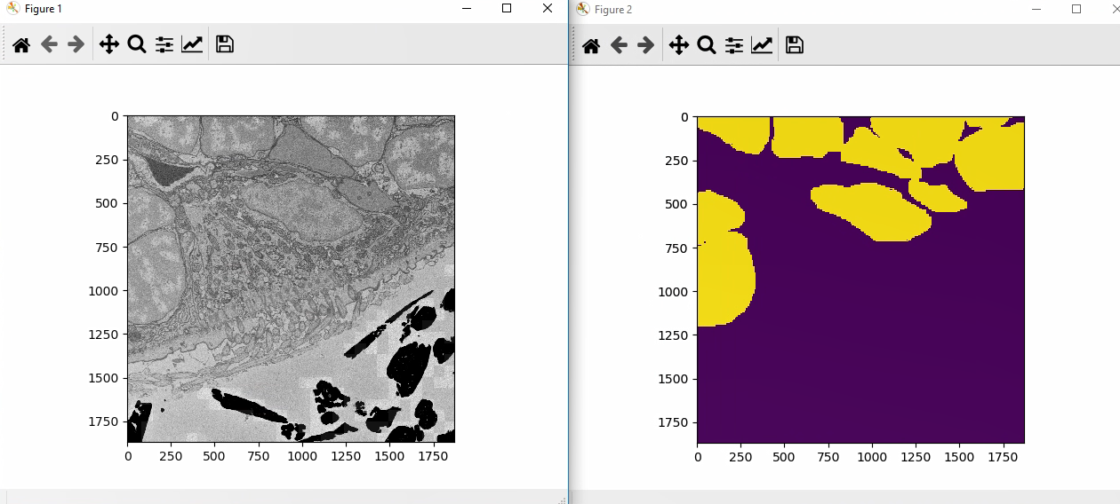
The ‘raw’ image is an electron microscopy image of cells from the marine worm Platynereis dumerilii. The ‘nuclei’ image is a segmentation of the nuclei of these same cells.

The Basic Features of NumPy Arrays

Once we have our data in a NumPy array, we want to explore it a bit e.g. how many dimensions does our array have, and of what size? This is represented by the shape of an array, which denotes the length of the array in each dimension. Returning to the toy arrow example above:

print(arrow.shape)
print(arrow.ndim)

# the image is 4 pixels by 4 pixels
(4, 4)
# the image is 2D
2

We might also want to know what type of data is inside our array? This can be accessed in a similar way to the shape of the array, but now using the dtype attribute (we’ll expand on data types in a later section).

Finally, we might want to calculate some summary statistics for our array like the mean or standard deviation.

print(np.mean(raw))
print(np.std(raw))

158.46056878949926
46.708246304034866

2.1. Exploring Image Arrays

What are the dimensions of the raw and nuclei arrays?

What data type are these arrays?

What is the minimum and maximum value of these arrays?
Solution
print(raw.shape)
print(raw.dtype)
print(np.max(raw))
print(np.min(raw))

Indexing Arrays

Now we have a general idea of what our array contains, we want to start manipulating particular regions of it.

We can index arrays by the integer location on each axis. e.g. for 2D arrays, (0,0) is the top left of the image. The first value is the index of the rows in the image, and the second is the index of the columns: (row, column)

# access the value at (0,0)
print(raw[0,0])

We can use slicing to access multiple elements at once e.g.

# get part of array from rows 3-6 and columns 4-7
# (note the top end of these slices are non-inclusive)
print(raw[3:7,4:8])

# we can get the whole of an axis by just using ':' e.g. here we get the whole of the third row
print(raw[3, :])

array([[156, 173, 156, 161],
       [145, 183, 152, 147],
       [165, 166, 161, 159],
       [160, 156, 150, 167]], dtype=uint8)

[154 160 150 ... 102 101 111]

2.2. Subsetting a NumPy Array

Crop the ‘raw’ image, by removing a border of 500 pixels on all sides.

Solution

border_size = 500
new_image = raw[border_size:raw.shape[0]-border_size, border_size:raw.shape[1]-border_size]
# We could have also written
# new_image = raw[border_size:-border_size, border_size:-border_size]
# making use of python negative indexing - i.e. from the end of the array - works on lists too
plt.imshow(new_image, cmap='gray')

Boolean Indexing

Sometimes we want to access certain parts of an array not based on position, but instead on some criterion. e.g. selecting values that are above some threshold.

We can do this simply with Boolean indexing in NumPy. As an example, let’s find all pixels with a value greater than 100:

criteria = raw > 100
print(criteria)
print(criteria.shape)

[[ True  True  True ...  True  True  True]
 [ True  True  True ...  True  True False]
 [ True  True  True ...  True  True  True]
 ...
 [False False False ... False False False]
 [False False False ... False False False]
 [False False False ... False False False]]

 (1870, 1870)

We see that this operation creates a Boolean NumPy array with the same shape as the original raw array. (A Boolean array is populated with True and False values.) We can use this directly for indexing! This will keep elements where there is True and discard those with False.

print(raw[criteria])

array([132, 164, 175, ..., 200, 174, 109], dtype=uint8)

We can use this logic to select elements under various more complicated criteria e.g. combining different criteria with & (and) and | (or). Let’s select elements that are greater than 100 and smaller than 200:

criteria = (raw > 100) & (raw < 200)
print(raw[criteria])

[132 164 175 ... 189 174 109]

2.3. Masking Arrays

The nuclei image contains a binary segmentation i.e.:

1 = nuclei

0 = not nuclei

Find the median value of the raw image within the nuclei

Create a new version of raw where all values outside the nuclei are 0
Solution
# 1
pixels_in_nuclei = raw[nuclei == 1]
print(np.median(pixels_in_nuclei))

# 2
new_image = raw.copy()
new_image[nuclei == 0] = 0
plt.imshow(new_image, cmap='gray')

The Power of Vectorisation

One of the big advantages of NumPy is that operations are vectorised. This means that operations can be applied to the whole array very quickly, without the need for loops. Many of the operations we’ve used so far are vectorised! But let’s look at a more specific example to make this point more clearly:

Say we want to make a new image where all values are 5 less than before. We could do this with a for loop:

new_image = raw.copy()
for i in range(0, raw.shape[0]):
    for j in range(0, raw.shape[1]):
        new_image[i, j] = raw[i, j] - 5

This works fine, but we could do this in one-line in NumPy!

new_image = raw - 5

All the standard operations e.g. +, -, * etc will be applied elementwise, to every element in a NumPy array. This allows you to replace many complex loops with one line statments, and also makes for very fast computation.

Many standard maths operations are also implemented in NumPy e.g.

np.cos(2)
np.sin(2)
np.exp(2)

NumPy Data Types

As we touched on briefly earlier, each ndarray has a particular data type (dtype) assigned to it. This defines what kind of values (and what range of values) can be placed in the array. e.g. int8, uint16, float64…

We can find the data type of our array, and change it, like so:

# print current data type
print(nuclei.dtype)

# change the data type
print((nuclei.astype('uint16')).dtype)

uint8
uint16

The names of these data types consist of two parts:

The kind of data allowed e.g. int = integer, uint = unsigned integer (i.e. no negative values), float = floating point numbers
The bitsize - e.g. 8-bit, 16-bit, 64-bit…

The bitsize relates to how that particular element is stored in your computer’s memory. A larger bitsize allows you to store a wider range of values, but will take up more space. Choosing the bitsize is always a trade-off between the space it takes up in your computer’s memory, and the size of the numbers you want to store. Note that the size of the values stored in the array has little effect on the memory it takes up i.e. an array of small values but with a large bitsize will still take up a lot of memory.

2.4. Working with Data Types

Increase the brightness of the image by 100

Why does the result look so bizarre? What is going wrong here?

How would you fix this issue?
Solution
# 1
new_image = raw + 100
plt.imshow(new_image, cmap='gray')
# 2
print(raw.dtype)
print(np.max(raw))
# The data type is 'uint8' i.e. unsigned 8 bit integer (max value 255)
# When 100 is added, many values overflow, giving unexpected results

# 3
new_raw = raw.astype('uint32')
plt.imshow(new_raw + 100, cmap='gray')

If you want to learn more about NumPy, a good place to start is their docs - they’ve written a number of tutorials to get you started!

pandas

To explore the power of the pandas library, we will work with a different dataset: one that combines numeric and non-numeric data. As with the ndarray object in NumPy, the central object in pandas is the DataFrame which we will work with throughout this section. The DataFrame can efficiently handle quantitative data (e.g. integers and floats) together with qualititative data (e.g. categoricals such as sample-IDs or species names), and comes packed with features to help analyse and summarise that data.

Loading Data

To get started with pandas, let’s import the module (giving it a nice, short name to save us some keystrokes) and use the read_csv function to create our first DataFrame object. (You can download the data file here: data/CovidCaseData_20200705.csv. The code examples assume that you save these files in a folder called data.)

import pandas as pd   # this is how pandas is traditionally imported
covid_cases = pd.read_csv("data/CovidCaseData_20200705.csv")

From the filename, we can guess a little bit about what is described in the dataset we’ve loaded. To get a quick visual overview of the new dataframe, we can print it:

print(covid_cases)

          dateRep  day  month  year  cases  deaths countriesAndTerritories  \
    05/07/2020    5      7  2020    348       7             Afghanistan
    04/07/2020    4      7  2020    302      12             Afghanistan
    03/07/2020    3      7  2020    186      33             Afghanistan
    02/07/2020    2      7  2020    319      28             Afghanistan
    01/07/2020    1      7  2020    279      13             Afghanistan
...           ...  ...    ...   ...    ...     ...                     ...
25/03/2020   25      3  2020      0       0                Zimbabwe
24/03/2020   24      3  2020      0       1                Zimbabwe
23/03/2020   23      3  2020      0       0                Zimbabwe
22/03/2020   22      3  2020      1       0                Zimbabwe
21/03/2020   21      3  2020      1       0                Zimbabwe

geoId countryterritoryCode  popData2019 continentExp
      AF                  AFG   38041757.0         Asia
      AF                  AFG   38041757.0         Asia
      AF                  AFG   38041757.0         Asia
      AF                  AFG   38041757.0         Asia
      AF                  AFG   38041757.0         Asia
...     ...                  ...          ...          ...
  ZW                  ZWE   14645473.0       Africa
  ZW                  ZWE   14645473.0       Africa
  ZW                  ZWE   14645473.0       Africa
  ZW                  ZWE   14645473.0       Africa
  ZW                  ZWE   14645473.0       Africa

[27831 rows x 11 columns]

From this output, we can already get a feeling for the data we’ve loaded:

it has >27,800 rows and 11 columns
the data in these columns include integers (day-of-month, number of cases, etc), floating point numbers (population of country in 2019), and non-numeric data (dates, continent and country names, etc)
the rows seem to be indexed numerically starting from 0
the dataframe includes data from at least two countries (Afghanistan and Zimbabwe) and continents (Asia and Africa).
- based on the appearance of Afghanistan at the top of the dataframe, and Zimbabwe at the bottom, we may assume that countries are ordered alphabetically though we aren’t yet able to understand all the details of that ordering

Jupyter 🧡 pandas

Jupyter provides a very friendly environment for working with dataframes: users can take advantage of the way that Jupyter displays the value from the last line in an executed cell to access a more visually-pleasing display than we got from print above.

Remember that, unless you explicitly call print on additional lines, Jupyter only shows you the value from the last line of a cell:

Working with Dataframes

All those ... in the output from print above indicate that some lines were skipped to display a truncated view of the dataframe. For such a large dataset, it’s unhelpful to view the entire thing at once. For convenience, DataFrame objects are equipped with head and tail methods that allow us to view only the first or last handful of rows respectively. (If you use the UNIX Shell, you may already be familiar with the commands these methods are named after.)

print(covid_cases.head())

      dateRep  day  month  year  cases  deaths countriesAndTerritories geoId countryterritoryCode  popData2019 continentExp
05/07/2020    5      7  2020    348       7             Afghanistan    AF                  AFG   38041757.0         Asia
04/07/2020    4      7  2020    302      12             Afghanistan    AF                  AFG   38041757.0         Asia
03/07/2020    3      7  2020    186      33             Afghanistan    AF                  AFG   38041757.0         Asia
02/07/2020    2      7  2020    319      28             Afghanistan    AF                  AFG   38041757.0         Asia
01/07/2020    1      7  2020    279      13             Afghanistan    AF                  AFG   38041757.0         Asia

covid_cases.tail()

          dateRep  day  month  year  cases  deaths countriesAndTerritories geoId countryterritoryCode  popData2019 continentExp
25/03/2020   25      3  2020      0       0                Zimbabwe    ZW                  ZWE   14645473.0       Africa
24/03/2020   24      3  2020      0       1                Zimbabwe    ZW                  ZWE   14645473.0       Africa
23/03/2020   23      3  2020      0       0                Zimbabwe    ZW                  ZWE   14645473.0       Africa
22/03/2020   22      3  2020      1       0                Zimbabwe    ZW                  ZWE   14645473.0       Africa
21/03/2020   21      3  2020      1       0                Zimbabwe    ZW                  ZWE   14645473.0       Africa

# provide an integer argument to head or tail to specify the number of rows to display
print(covid_cases.head(1))

      dateRep  day  month  year  cases  deaths countriesAndTerritories geoId countryterritoryCode  popData2019 continentExp
0  05/07/2020    5      7  2020    348       7             Afghanistan    AF                  AFG   38041757.0         Asia

As we’ll see later, it can sometimes be helpful to quickly access basic information about a dataframe. DataFrame objects carry a lot of useful information about themselves around as attributes. For example, we can use the shape attribute to see the dimensions of the dataframe, and the names of its columns via the columns attribute:

print(f'covid_cases is a {type(covid_cases)} object with {covid_cases.shape[0]} rows and {covid_cases.shape[1]} columns')
print('covid_cases has the following columns:\n' + '\n'.join(covid_cases.columns))

covid_cases is a <class 'pandas.core.frame.DataFrame'> object with 27831 rows and 11 columns
covid_cases has the following columns:
dateRep
day
month
year
cases
deaths
countriesAndTerritories
geoId
countryterritoryCode
popData2019
continentExp

However, if you want the kind of summary we’ve created above, it’s much easier to use covid_cases.info():

print(covid_cases.info())

<class 'pandas.core.frame.DataFrame'>
RangeIndex: 27831 entries, 0 to 27830
Data columns (total 11 columns):
 #   Column                   Non-Null Count  Dtype
---  ------                   --------------  -----
 0   dateRep                  27831 non-null  object
 1   day                      27831 non-null  int64
 2   month                    27831 non-null  int64
 3   year                     27831 non-null  int64
 4   cases                    27831 non-null  int64
 5   deaths                   27831 non-null  int64
 6   countriesAndTerritories  27831 non-null  object
 7   geoId                    27718 non-null  object
 8   countryterritoryCode     27767 non-null  object
 9   popData2019              27767 non-null  float64
 10  continentExp             27831 non-null  object
dtypes: float64(1), int64(5), object(5)
memory usage: 2.3+ MB

From this output, we can learn a few more things about our dataset:

8 of the 11 columns have 27,831 non-null values, meaning that these columns contain no missing data
two columns (countryterritoryCode and popData2019) have 27,767 non-null values, meaning they are missing data in 64 rows
the geoId column is missing data in 113 rows
the values in the integer & float columns are stored at 64 bit precision
the dataframe is using roughly 2.1 MB of memory on the system

We’ll return to that missing data later. For now, let’s finish our tour of the descriptive features of DataFrame objects by looking at the describe method, which provides an overview of the distribution of values in all the quantitative columns in the dataframe:

print(covid_cases.describe())

                day         month          year         cases        deaths   popData2019
count  27831.000000  27831.000000  27831.000000  27831.000000  27831.000000  2.776700e+04
mean      15.814811      4.312996   2019.997593    403.925658     19.067515  4.640626e+07
std        8.994855      1.617419      0.049007   2351.306962    120.833161  1.664285e+08
min        1.000000      1.000000   2019.000000 -29726.000000  -1918.000000  8.150000e+02
25%        8.000000      3.000000   2020.000000      0.000000      0.000000  1.798506e+06
50%       16.000000      4.000000   2020.000000      4.000000      0.000000  8.776119e+06
75%       24.000000      6.000000   2020.000000     72.000000      1.000000  3.182530e+07
max       31.000000     12.000000   2020.000000  54771.000000   4928.000000  1.433784e+09

By viewing the minimum, maximum, and quartile values for each column, we can quickly get an idea for the shape of our data and perhaps spot something that looks weird. Of course, in some cases, like the day, month, and year columns here, numbers such as the mean and standard deviation aren’t helpful. In such situations, it’s up to you as the user to make the distinction between the meaningful and meaningless.

Selecting Data in a Dataframe

Viewing and browsing the dataframe as a whole is a way to get a high-level understanding of the kind of data we’re working with and to run a quick “sniff test” to get an idea of what issues might be present. But at some stage, we have to start digging down into specific columns, rows, and cells to be able to access the information we need.

To select one or more specific cells from a dataframe, use the iloc & loc methods with [] square brackets containing the coordinates. iloc expects the coordinate references as integers:

print(covid_cases.iloc[22222,4])

# to get an entire row, leave the column coordinate blank...
print(covid_cases.iloc[24242,], '\n')

dateRep                      06/05/2020
day                                   6
month                                 5
year                               2020
cases                              1595
deaths                                9
countriesAndTerritories    Saudi_Arabia
geoId                                SA
countryterritoryCode                SAU
popData2019                 3.42685e+07
continentExp                       Asia
Name: 22222, dtype: object

Whereas loc expects to receive row/column names. (The rows in the dataframe we’re working with right now are indexed numerically, so we can’t use names for these yet.)

print(covid_cases.loc[20000,'cases'])

DataFrame ≠ ndarray

Unlike the NumPy array, we can’t access individual positions of a DataFrame object by directly referring to the coordinates we’re interested in, e.g. covid_cases[100,0] raises a KeyError.

If you’d like to select a range of rows or columns, you can use slices with iloc & loc:

print('covid_cases.iloc[100:105,4:6]')
print(covid_cases.iloc[100:105,4:6])

print('\ncovid_cases.iloc[100:105,:]')
print(covid_cases.iloc[100:105,:])

print('\nselect a whole row:')
print(covid_cases.loc[0,:])
# or
print(covid_cases.loc[0,])

print('\nselect a whole column:')
print(covid_cases.loc[:,'continentExp'])
# or
print(covid_cases['continentExp'])
# or(!)
print(covid_cases.continentExp)

print('\nWarning! Numeric ranges and named slices behave differently:')
print('range with numeric indices: covid_cases.loc[1500:1510, 1:3]')
print(covid_cases.iloc[1500:1510, 1:3]) # doesn't include year (fourth) column
print('range with named indices: covid_cases.loc[1500:1510, "day":"year"]')
print(covid_cases.loc[1500:1510, "day":"year"]) # includes year column

covid_cases.iloc[100:105,4:6]
     cases  deaths
100      0       0
101     33       0
102      2       0
103      6       1
104     10       0

covid_cases.iloc[100:105,:]
        dateRep  day  month  year  cases  deaths countriesAndTerritories geoId countryterritoryCode  popData2019 continentExp
100  27/03/2020   27      3  2020      0       0             Afghanistan    AF                  AFG   38041757.0         Asia
101  26/03/2020   26      3  2020     33       0             Afghanistan    AF                  AFG   38041757.0         Asia
102  25/03/2020   25      3  2020      2       0             Afghanistan    AF                  AFG   38041757.0         Asia
103  24/03/2020   24      3  2020      6       1             Afghanistan    AF                  AFG   38041757.0         Asia
104  23/03/2020   23      3  2020     10       0             Afghanistan    AF                  AFG   38041757.0         Asia

select a whole row:
dateRep                     05/07/2020
day                                  5
month                                7
year                              2020
cases                              348
deaths                               7
countriesAndTerritories    Afghanistan
geoId                               AF
countryterritoryCode               AFG
popData2019                3.80418e+07
continentExp                      Asia
Name: 0, dtype: object
dateRep                     05/07/2020
day                                  5
month                                7
year                              2020
cases                              348
deaths                               7
countriesAndTerritories    Afghanistan
geoId                               AF
countryterritoryCode               AFG
popData2019                3.80418e+07
continentExp                      Asia
Name: 0, dtype: object

select a whole column:
0          Asia
1          Asia
2          Asia
3          Asia
4          Asia
          ...
27826    Africa
27827    Africa
27828    Africa
27829    Africa
27830    Africa
Name: continentExp, Length: 27831, dtype: object
0          Asia
1          Asia
2          Asia
3          Asia
4          Asia
          ...
27826    Africa
27827    Africa
27828    Africa
27829    Africa
27830    Africa
Name: continentExp, Length: 27831, dtype: object
0          Asia
1          Asia
2          Asia
3          Asia
4          Asia
          ...
27826    Africa
27827    Africa
27828    Africa
27829    Africa
27830    Africa
Name: continentExp, Length: 27831, dtype: object

Warning! Numeric ranges and named slices behave differently:
range with numeric indices: covid_cases.loc[1500:1510, 1:3]
      day  month
1500    1      1
1501   31     12
1502    5      7
1503    4      7
1504    3      7
1505    2      7
1506    1      7
1507   30      6
1508   29      6
1509   28      6
range with named indices: covid_cases.loc[1500:1510, "day":"year"]
      day  month  year
1500    1      1  2020
1501   31     12  2019
1502    5      7  2020
1503    4      7  2020
1504    3      7  2020
1505    2      7  2020
1506    1      7  2020
1507   30      6  2020
1508   29      6  2020
1509   28      6  2020
1510   27      6  2020

If you select all or part of a single column, it is returned as a pandas Series object. This is similar to a one-dimensional ndarray, but with a named index.

print(type(covid_cases['continentExp']))

<class 'pandas.core.series.Series'>

Let’s take the continentExp column as an example, then use the values in that column to get a better idea of how much of the world is accounted for in our data. To access the unique values in this column, we can call its unique method, or the unique function that pandas provides:

print(covid_cases['continentExp'].unique())
# equivalent to pd.unique(covid_cases['continentExp'])

array(['Asia', 'Europe', 'Africa', 'America', 'Oceania', 'Other'],
      dtype=object)

From this, we can see that our covid_cases dataframe contains data for countries in five landmasses - Africa, America (North & South combined), Asia, Europe, and Oceania - and a mysterious “Other” category. We can also see that the unique method returned the values in an ndarray.

Filtering Data in a Dataframe

So now we’ve seen how to access specific positions, and ranges of positions, in a dataframe. This can be very useful for exploration of a dataset, or creating a simple subset e.g. for testing purposes (though we would recommend you take a random subset from the dataframe with the sample method for that purpose).

When exploring and processing large datasets, it’s typically much more helpful to be able to select and filter data based on the values found in a particular column.

For example, now that we’ve seen the unique values present in the continentExp column of covid_cases, we might be interested to investigate the rows categorised under “Other”. To do this, we take a similar approach to the masking we saw with NumPy earlier:

print(covid_cases['continentExp'] == 'Other')
print('\nUsing this comparison to filter out rows not containing "Other" in the "continentExp" column:')
print(covid_cases[covid_cases['continentExp'] == 'Other'])

      False
      False
      False
      False
      False
         ...
  False
  False
  False
  False
  False
Name: continentExp, Length: 27831, dtype: bool

Using this comparison to filter out rows not containing "Other" in the "continentExp" column:
         dateRep  day  month  year  ...     geoId  countryterritoryCode popData2019 continentExp
10/03/2020   10      3  2020  ...  JPG11668                   NaN         NaN        Other
02/03/2020    2      3  2020  ...  JPG11668                   NaN         NaN        Other
01/03/2020    1      3  2020  ...  JPG11668                   NaN         NaN        Other
29/02/2020   29      2  2020  ...  JPG11668                   NaN         NaN        Other
28/02/2020   28      2  2020  ...  JPG11668                   NaN         NaN        Other
...          ...  ...    ...   ...  ...       ...                   ...         ...          ...
04/01/2020    4      1  2020  ...  JPG11668                   NaN         NaN        Other
03/01/2020    3      1  2020  ...  JPG11668                   NaN         NaN        Other
02/01/2020    2      1  2020  ...  JPG11668                   NaN         NaN        Other
01/01/2020    1      1  2020  ...  JPG11668                   NaN         NaN        Other
31/12/2019   31     12  2019  ...  JPG11668                   NaN         NaN        Other

[64 rows x 11 columns]

The output above shows us that the comparison covid_cases['continentExp'] == 'Other' returns a series of Booleans. Applying this series to the whole dataframe returns a view of the dataframe that contains only the rows corresponding to the True values from the comparison. Unfortunately, the truncated output (with some columns not displayed) doesn’t give us much insight into what these rows describe - the geoId ‘JPG11668’ isn’t particularly informative…

2.5. What’s going on?

Take a look at the names of all the columns in covid_cases and choose one that gives you a better understanding of where the data in these rows has come from. (Hint: the dataframe view returned by a filtering like the one above can be treated just like a complete dataframe.)
Solution
print(covid_cases.columns) # see the column names
# display only the unique values from the "countriesAndTerritories" column
# in the filtered data
print(covid_cases[covid_cases['continentExp'] == 'Other']['countriesAndTerritories'].unique())
Index(['dateRep', 'day', 'month', 'year', 'cases', 'deaths',
       'countriesAndTerritories', 'geoId', 'countryterritoryCode',
       'popData2019', 'continentExp'],
      dtype='object')
['Cases_on_an_international_conveyance_Japan']
The cases described in these rows were detected on a cruise ship off the coast of Japan.

One other thing we could see from the filtering above, is that these rows also account for the 64 missing values we identified in the countryterritoryCode and popData2019 columns when we inspected the output of covid_cases.info().

Accidentally Omitted Data

What about those 113 rows we found were missing a value in the geoId column? To pull these rows out of the dataframe, we can use the isna function from pandas, which returns True for fields with NaN (null) values, and False otherwise:

print(covid_cases[pd.isna(covid_cases['geoId'])])

          dateRep  day  month  year  cases  deaths countriesAndTerritories geoId countryterritoryCode  popData2019 continentExp
05/07/2020    5      7  2020     25       0                 Namibia   NaN                  NAM    2494524.0       Africa
04/07/2020    4      7  2020     57       0                 Namibia   NaN                  NAM    2494524.0       Africa
03/07/2020    3      7  2020      8       0                 Namibia   NaN                  NAM    2494524.0       Africa
02/07/2020    2      7  2020     82       0                 Namibia   NaN                  NAM    2494524.0       Africa
01/07/2020    1      7  2020      7       0                 Namibia   NaN                  NAM    2494524.0       Africa
...           ...  ...    ...   ...    ...     ...                     ...   ...                  ...          ...          ...
19/03/2020   19      3  2020      0       0                 Namibia   NaN                  NAM    2494524.0       Africa
18/03/2020   18      3  2020      0       0                 Namibia   NaN                  NAM    2494524.0       Africa
17/03/2020   17      3  2020      0       0                 Namibia   NaN                  NAM    2494524.0       Africa
16/03/2020   16      3  2020      0       0                 Namibia   NaN                  NAM    2494524.0       Africa
15/03/2020   15      3  2020      2       0                 Namibia   NaN                  NAM    2494524.0       Africa

[113 rows x 11 columns]

This shows that the 113 rows in question are data about from Namibia. Closer inspection of the source data shows us that the problem is the two-letter code, ‘NA’, being used to represent Namibia in the geoId column. By default, the read_csv function we used to load the data processes ‘NA’ as having the special meaning “missing/null value”, and converts these to NaN in the resulting DataFrame! (It’s important to be aware of special behaviour like this, which functions like read_csv have because they match the expectations/desired behaviour of the user in the majority of cases - we probably should’ve read about all the options and their defaults in the documentation before we called the function…) This hasn’t caused a problem so far, but could easily confound downstream analyses, so let’s fix the issue.

We haven’t modified the dataframe since it was first loaded, so the easiest thing to do here is simply to reload the data. The options we need to change are na_values, which by default is set to interpret a whole host of values as meaning NaN, and keep_default_na, which is a Boolean switch telling read_csv whether to append our the NaN values we specify with na_values to the default set it would use anyway (True), or whether to use only the set of values we specified (False). To process only empty values ('') as NaN, we can run read_csv like this:

covid_cases = pd.read_csv('data/CovidCaseData_20200705.csv', na_values=[''], keep_default_na=False)
print(covid_cases[pd.isna(covid_cases['geoId'])])

Empty DataFrame
Columns: [dateRep, day, month, year, cases, deaths, countriesAndTerritories, geoId, countryterritoryCode, popData2019, continentExp]
Index: []

Great, now that we’re finally working with a cleaned up dataframe, we can get back on with exploring it.

Advanced Filtering

We can combine multiple criteria when filtering a dataframe, placing each comparison in a set of () parentheses and combining them with & (logical AND) or | (logical OR). For example, you might want to select only the rows for April in Denmark:

mask = (covid_cases['month'] == 4) & (covid_cases['countryterritoryCode'] == 'DNK')
print(covid_cases[mask])
# or the equivalent, all in one long line:
# print(covid_cases[(covid_cases['month'] == 4) & (covid_cases['countryterritoryCode'] == 'DNK')])

         dateRep  day  month  year  cases  deaths countriesAndTerritories geoId countryterritoryCode  popData2019 continentExp
30/04/2020   30      4  2020    157       9                 Denmark    DK                  DNK    5806081.0       Europe
29/04/2020   29      4  2020    153       7                 Denmark    DK                  DNK    5806081.0       Europe
28/04/2020   28      4  2020    123       5                 Denmark    DK                  DNK    5806081.0       Europe
27/04/2020   27      4  2020    130       4                 Denmark    DK                  DNK    5806081.0       Europe
26/04/2020   26      4  2020    235      15                 Denmark    DK                  DNK    5806081.0       Europe
25/04/2020   25      4  2020    137       9                 Denmark    DK                  DNK    5806081.0       Europe
24/04/2020   24      4  2020    161      10                 Denmark    DK                  DNK    5806081.0       Europe
23/04/2020   23      4  2020    217      14                 Denmark    DK                  DNK    5806081.0       Europe
22/04/2020   22      4  2020    180       6                 Denmark    DK                  DNK    5806081.0       Europe
21/04/2020   21      4  2020    131       9                 Denmark    DK                  DNK    5806081.0       Europe
20/04/2020   20      4  2020    142       9                 Denmark    DK                  DNK    5806081.0       Europe
19/04/2020   19      4  2020    169      10                 Denmark    DK                  DNK    5806081.0       Europe
18/04/2020   18      4  2020    194      15                 Denmark    DK                  DNK    5806081.0       Europe
17/04/2020   17      4  2020    198      12                 Denmark    DK                  DNK    5806081.0       Europe
16/04/2020   16      4  2020    170      10                 Denmark    DK                  DNK    5806081.0       Europe
15/04/2020   15      4  2020    193      14                 Denmark    DK                  DNK    5806081.0       Europe
14/04/2020   14      4  2020    144      12                 Denmark    DK                  DNK    5806081.0       Europe
13/04/2020   13      4  2020    178      13                 Denmark    DK                  DNK    5806081.0       Europe
12/04/2020   12      4  2020    177      13                 Denmark    DK                  DNK    5806081.0       Europe
11/04/2020   11      4  2020    184      10                 Denmark    DK                  DNK    5806081.0       Europe
10/04/2020   10      4  2020    233      19                 Denmark    DK                  DNK    5806081.0       Europe
09/04/2020    9      4  2020    331      15                 Denmark    DK                  DNK    5806081.0       Europe
08/04/2020    8      4  2020    390      16                 Denmark    DK                  DNK    5806081.0       Europe
07/04/2020    7      4  2020    312       8                 Denmark    DK                  DNK    5806081.0       Europe
06/04/2020    6      4  2020    292      18                 Denmark    DK                  DNK    5806081.0       Europe
05/04/2020    5      4  2020    320      22                 Denmark    DK                  DNK    5806081.0       Europe
04/04/2020    4      4  2020    371      16                 Denmark    DK                  DNK    5806081.0       Europe
03/04/2020    3      4  2020    279      19                 Denmark    DK                  DNK    5806081.0       Europe
02/04/2020    2      4  2020    247      14                 Denmark    DK                  DNK    5806081.0       Europe
01/04/2020    1      4  2020    283      13                 Denmark    DK                  DNK    5806081.0       Europe

2.6. Filtering Practice

Use what you’ve learned to find all rows in the covid_cases dataframe that report cases in the year 2019.

Solution

mask = (covid_cases['cases'] > 1) & (covid_cases['year'] == 2019)
print(covid_cases[mask])

         dateRep  day  month  year  ...  geoId  countryterritoryCode   popData2019 continentExp
5643  31/12/2019   31     12  2019  ...     CN                   CHN  1.433784e+09         Asia

[1 rows x 11 columns]

The results of filtering are provided as a view of the dataframe, which means they can be used in further operations. For example, we might want to find the maximum number of cases reported on a single day in Europe:

covid_cases[covid_cases['continentExp'] == 'Europe']['cases'].max()

2.7. Working with Filtered Data

On what date were the most cases reported in Germany so far?
What was the mean number of cases reported per day in Germany in April 2020?
Is this higher or lower than the mean for March 2020?
On how many days in March was the number of cases in Germany higher than the mean for April?

Solution

# 1
mask_germany = covid_cases['countryterritoryCode'] == 'DEU'
id_max = covid_cases[mask_germany]['cases'].idxmax()
print(covid_cases.iloc[id_max]['dateRep'])

# 2
mask_april = (covid_cases['year'] == 2020) & (covid_cases['month'] == 4)
mean_april = covid_cases[mask_germany & mask_april]['cases'].mean()
print(mean_april)

# 3
mask_march = (covid_cases['year'] == 2020) & (covid_cases['month'] == 3)
mean_march = covid_cases[mask_germany & mask_march]['cases'].mean()
print(mean_march)
print("Mean cases per day was {} in April than in March 2020.".
      format(["lower", "higher"][mean_april > mean_march]))

# 4
mask_higher_mean_april = (covid_cases['cases'] > mean_april)
selection = covid_cases[mask_germany & mask_march & mask_higher_mean_april]
nbr_days = len(selection)   # Assume clean data
print(nbr_days)

Combining Dataframes

Before we can explore how to combine data from multiple dataframes, we first need to load in some additional data.

You can download the data files here:

(The code examples assume that you save these files in a folder called data.)

The first (left-most) column in the datasets we’ll use now is full of unique values, which means we can use this column as the index for the dataset we’ll create when we load it in. This index can then be used to refer to rows by the value they have in the index, rather than numerically as we’ve been doing up to now. To set this index when we load the data, we use the index_col parameter, indicating that we want to use the first column as the index:

asia_lockdowns = pd.read_csv('data/AsiaLockdowns.csv', index_col=0)
africa_lockdowns = pd.read_csv('data/AfricaLockdowns.csv', index_col=0)
print(asia_lockdowns.head())
print(africa_lockdowns.head())

                           Start date    End date
Countries and territories
Bangladesh                 2020-03-26  2020-05-16
India                      2020-03-25  2020-06-30
Iran                       2020-03-14  2020-04-20
Iraq                       2020-03-22  2020-04-11
Israel                     2020-04-02         NaN
                           Start date    End date
Countries and territories
Algeria                    2020-03-23  2020-05-14
Botswana                   2020-04-02  2020-04-30
Congo                      2020-03-31  2020-04-20
Eritrea                    2020-04-02  2020-04-23
Ghana                      2020-03-30  2020-04-12

Note how the two dataframes we’ve just loaded have the same structure - two data columns, Start date and End date and an index of country/territory names - only the values within therein are different between the two.

Now that we’ve got a couple dataframes with a non-numeric index, let’s briefly revisit the loc method of the DataFrame object. Remember that we could select columns by name with this method? We can do the same with the rows in these dataframes:

print('Selecting all columns for a named row:')
print(africa_lockdowns.loc['Eritrea',])
print('\n...and one column for a range of rows:')
print(asia_lockdowns.loc['Iran':'Nepal','Start date'])

Selecting all columns for a named row:
Start date    2020-04-02
End date      2020-04-23
Name: Eritrea, dtype: object

...and one column for a range of rows:
Countries and territories
Iran        2020-03-14
Iraq        2020-03-22
Israel      2020-04-02
Jordan      2020-03-18
Kuwait      2020-03-14
Lebanon     2020-03-15
Malaysia    2020-03-18
Mongolia    2020-03-10
Nepal       2020-03-24
Name: Start date, dtype: object

(Note that the first filtering, selecting all columns for the “Eritrea” row, returned a Series object as the data is one-dimensional.)

Our other dataframe (the one we loaded in when we first began working with pandas) contains data for the whole world. So it would be good to collect all this lockdown data into a single dataframe too, before finally combining it all together.

We can use the concat function to concatenate the two new dataframes together. It’s a straightforward operation - adding the rows from one to the bottom of the other - because the two dataframes have the same column structure.

concatenated = pd.concat([africa_lockdowns, asia_lockdowns])
print(concatenated.iloc[10:21,])

                           Start date    End date
Countries and territories
Nigeria                    2020-03-30  2020-04-12
Papua_New_Guinea           2020-03-24  2020-04-07
Rwanda                     2020-03-21  2020-04-19
South_Africa               2020-03-26  2020-04-30
Tunisia                    2020-03-22  2020-04-19
Zimbabwe                   2020-03-30  2020-05-02
Bangladesh                 2020-03-26  2020-05-16
India                      2020-03-25  2020-06-30
Iran                       2020-03-14  2020-04-20
Iraq                       2020-03-22  2020-04-11
Israel                     2020-04-02         NaN

2.8. Concatenating Dataframes

Load in the remaining lockdown data for the other continents (America, Europe, and Oceania) and concatenate all these sets of lockdown data together into a single dataframe called covid_lockdowns.
Solution
lockdown_dfs = [africa_lockdowns, asia_lockdowns]
for filename in ['data/AmericaLockdowns.csv', 'data/EuropeLockdowns.csv', 'data/OceaniaLockdowns.csv']:
    lockdown_dfs.append(pd.read_csv(filename, index_col="Countries and territories"))

covid_lockdowns = pd.concat(lockdown_dfs)

2.9. Working with an Indexed Dataframe

How many rows are in the covid_lockdowns dataframe?

On what date did lockdown begin in Lithuania?
Solution
# 1
print(f'covid_lockdowns has {covid_lockdowns.shape[0]} rows')

# 2
start_date_lithuania = covid_lockdowns.loc['Lithuania','Start date']
print(f'lockdowns began in Lithuania on {start_date_lithuania}')

Browsing this lockdown data, we can see missing values in the End date column. We guess (?) this indicates that these lockdowns hadn’t ended when this data was collected. However, these missing values could cause a problem downstream (for example, when we try to plot this data) so we should probably find a sensible way to fill them in. Let’s try to replace any missing values in the End date column with the most recent date included in the case data:

latest_date = covid_cases['dateRep'].max()
print(latest_date)

31/12/2019

Hmmmm. This doesn’t seem right, does it? Why does Python consider New Year’s Eve 2019 to be the maximum date in this column? To answer that question, we need to check the type of the data in that column:

print(covid_cases['dateRep'].dtype)

object

What does that mean now? Well, pandas stores columns with mixed types as objects. Are the entries maybe just strings? This would explain why we’re having troubles finding the ‘largest’ date

set([type(x) for x in covid_cases['dateRep']])

{<class 'str'>}

The values in the dateRep column of `covid_cases are being treated (and therefore sorted) as strings!

Working with Datetime Columns

Luckily, pandas provides an easy way to convert these to a datetime type, which can be handled and sorted correctly as dates:

pd.to_datetime(covid_cases['dateRep'], dayfirst=True)
# dayfirst=True is necessary because by default pandas reads mm/dd/yyyy dates :(
covid_cases['dateRep'] = pd.to_datetime(covid_cases['dateRep'], dayfirst=True)
print(covid_cases['dateRep'].max())

2020-07-05 00:00:00

This is much better! Now we can go back to what we were trying to do before: fill in those blank lockdown end dates with the latest date in covid_cases. We now know how to access the date we want to use to fill in missing values, but how can we efficiently find those missing values in the dataframe? Another DataFrame method fillna can give us what we need:

covid_lockdowns['End date'] = covid_lockdowns['End date']\
                                .fillna(covid_cases['dateRep'].max())
print(covid_lockdowns.info())

<class 'pandas.core.frame.DataFrame'>
Index: 89 entries, Algeria to Papua_New_Guinea
Data columns (total 2 columns):
 #   Column      Non-Null Count  Dtype
---  ------      --------------  -----
 0   Start date  89 non-null     object
 1   End date    89 non-null     object
dtypes: object(2)
memory usage: 2.1+ KB

Great! Now neither column is missing any data and we’re almost ready to move onto merging everything into one large dataset.

2.10. Practice with Datetime Conversions

Convert the “Start date” and “End date” columns in covid_lockdowns to datetime format. Note: watch out for how the dates are formatted in these columns! Is it the same as the format we saw in covid_cases['dateRep']?
Solution

The dates in these columns are written in an unambiguous format (yyyy-mm-dd), which pandas.to_datetime can convert without any additional information. In fact, for simple sorting purposes, dates represented this way as strings work just fine. This is one of several reasons why you should get into the habit of writing dates this way.
covid_lockdowns["Start date"] = pd.to_datetime(covid_lockdowns["Start date"])
covid_lockdowns["End date"] = pd.to_datetime(covid_lockdowns["End date"])

We saw earlier how to add rows to a dataframe with concat, and it’s also possible to add additional columns. The first option is to assign a Series to the dataframe, treating it like you might a dictionary and specifying the column name when you make the assignment:

covid_cases['casesPerMillion'] = covid_cases['cases'] / (covid_cases['popData2019']/1e6)
covid_cases.head()

     dateRep  day  month  year  cases  ...  geoId countryterritoryCode popData2019 continentExp  casesPerMillion
2020-07-05    5      7  2020    348  ...     AF                  AFG  38041757.0         Asia         9.147842
2020-07-04    4      7  2020    302  ...     AF                  AFG  38041757.0         Asia         7.938645
2020-07-03    3      7  2020    186  ...     AF                  AFG  38041757.0         Asia         4.889364
2020-07-02    2      7  2020    319  ...     AF                  AFG  38041757.0         Asia         8.385522
2020-07-01    1      7  2020    279  ...     AF                  AFG  38041757.0         Asia         7.334046

(Note that, if the series being assigned doesn’t have a length that matches the number of rows in the dataframe being assigned to, pandas will fill in the remaining space with NaNs.)

We can also use the DataFrame.merge method to add all the data from one dataframe into another. pandas figures out how to merge the data together based on matching up values in columns we can specify during the merge. It’s worth reading the documentation of merge (in fact, you’re going to have to in a moment, in order to complete an exercise) but, right now, suffice to say that we can merge on the index of covid_lockdowns and a column (countriesAndTerritories) of covid_cases provided that the names of the column & index match up:

covid_lockdowns.index.name='countriesAndTerritories'
combined = covid_cases.merge(covid_lockdowns, on="countriesAndTerritories")
print(combined.head())

     dateRep  day  month  year  cases  ...  popData2019 continentExp casesPerMillion  Start date    End date
2020-07-05    5      7  2020     67  ...    2862427.0       Europe       23.406710  2020-03-13  2020-06-01
2020-07-04    4      7  2020     90  ...    2862427.0       Europe       31.441850  2020-03-13  2020-06-01
2020-07-03    3      7  2020     82  ...    2862427.0       Europe       28.647019  2020-03-13  2020-06-01
2020-07-02    2      7  2020     45  ...    2862427.0       Europe       15.720925  2020-03-13  2020-06-01
2020-07-01    1      7  2020     69  ...    2862427.0       Europe       24.105418  2020-03-13  2020-06-01

[5 rows x 14 columns]

2.11. Joined in Hole-y Partnership

Compare the dimensions of the new combined dataframe with those of the original covid_cases dataframe. Do they match? If not, investigate combined, and the two dataframes from which it was created, to figure out why.

The merge method has a parameter, how, which is set to "inner" by default. Try out the other possible values ("outer", "left", and "right") and make sure you understand what’s going on in each case.

Solution

Using combined.shape, we can see that the new dataframe has many fewer rows than the original covid_cases. A closer inspection of covid_lockdowns shows us that there are a lot of countries and territories missing from that table, compared with the more comprehensive covid_cases list. This must be because these other countries haven’t put lockdowns in place (or perhaps that we just don’t have the data on those lockdowns). The data for these countries is not included in the combinded dataframe.

Where how="inner" only keeps rows with index values that appear in both merged dataframes, merging with how="outer" keeps all values in either index, inserting blank values (e.g. NaN) where no data can be included from one of the “parent” dataframes. how="left" and how="right" keep rows for all index values in either the first or the second dataframe in the merge call, respectively. As with "outer", blank values are inserted where data is missing in the other frame being merged.

Further Reading - Combining Series & Dataframes

For more on combining series and dataframes, we recommend these two chapters of Jake Vanderplas’ Python Data Science Handbook:

Combining Datasets: Concat and Append

Combining Datasets: Merge and Join

Groupby & Split-Apply-Combine

Everything we’re going to do in the rest of this chapter will concern only those countries and territories that appeared in both the covid_cases and covid_lockdowns dataframes, so we’ll keep working with the inner-joined combined dataframe.

It’s time to do a bit of actual data analysis, to demonstrate the power of pandas. Let’s calculate the average time, in days, between the beginning of a country’s lockdown, and the peak in new cases in that country. We’ll use the median time interval, to make the analysis more robust to outliers, and work with a rolling mean of case numbers (often referred to in the media as a moving average) to make our results less sensitive to daily fluctuations in case reports.

Before we can get the result we’re interested in, we need to overcome the following challenges:

The rows for each country/territory in the combined dataframe are currently sorted in descending date order (i.e. latest to earliest). We need to reverse this ordering, so that the rolling mean can be calculated correctly.
We need to find a way to calculate the rolling mean across the rows for each country, rather than over the dataframe as a whole.
The rolling mean values must be added as a new column in the dataframe.
We’ll have to find the peak of this rolling mean and calculate the time difference in days between that date and the respective lockdown start date for each country/territory.
Finally, we need to identify the median value of these time intervals.

Let’s tackle these challenges one at a time. From here on, we’re going to use an approach often referred to as split-apply-combine: first we split the data according to some criterion (in this case, the country or territory the row refers to), then we apply some function to each resulting group of data (that’s the rolling mean calculation and measuring the time interval), before finally combining the data back together to look at the complete results.

Step 1: If I Could Turn Back Time

pandas provides us with an easy way to reorder the rows in our dataframe. As you might have guessed by now, it’s another method of the DataFrame object: sort_values. As the name suggests, sort_values sorts the contents of the dataframe. It does so based on the values in the column(s) we specify with the by argument. We’d like to sort by two columns: countriesAndTerritories followed by dateRep.

print('before...')
print(combined.head(2))
combined = combined.sort_values(by=['countriesAndTerritories','dateRep'])
print('after...')
print(combined.head(2))

before...
     dateRep  day  month  year  cases  ...  popData2019 continentExp casesPerMillion  Start date    End date
0 2020-07-05    5      7  2020     67  ...    2862427.0       Europe        23.40671  2020-03-13  2020-06-01
1 2020-07-04    4      7  2020     90  ...    2862427.0       Europe        31.44185  2020-03-13  2020-06-01

[2 rows x 14 columns]
after...
       dateRep  day  month  year  cases  ...  popData2019 continentExp casesPerMillion  Start date    End date
118 2020-03-09    9      3  2020      2  ...    2862427.0       Europe        0.698708  2020-03-13  2020-06-01
117 2020-03-10   10      3  2020      4  ...    2862427.0       Europe        1.397416  2020-03-13  2020-06-01

[2 rows x 14 columns]

2. Like a Complete Unknown

Great! Everything is now set up for us to work on the rolling mean of cases for each country. As a first step, we need to divide up the dataframe based on the value in countriesAndTerritories, which means it’s time to introduce one of the DataFrame’s most powerful methods: groupby.

Calling groupby on a dataframe returns a special GroupBy object, which facilitates all kinds of useful things we might want to do with our grouped data. For example, we could group the data by continent, look at some information about the groups of data and display the country with the largest population for each continent:

continent_groups = combined.groupby('continentExp')
for continent, group_data in continent_groups:
    print(continent)
    print('type of group_data:', type(group_data))
    print('dimensions of group_data:', group_data.shape)
    maxidx = group_data['popData2019'].idxmax()
    print(group_data['countryterritoryCode'][maxidx], group_data['popData2019'][maxidx])

Africa
type of group_data: <class 'pandas.core.frame.DataFrame'>
dimensions of group_data: (1799, 14)
NGA 200963603.0
America
type of group_data: <class 'pandas.core.frame.DataFrame'>
dimensions of group_data: (2349, 14)
USA 329064917.0
Asia
type of group_data: <class 'pandas.core.frame.DataFrame'>
dimensions of group_data: (3700, 14)
IND 1366417756.0
Europe
type of group_data: <class 'pandas.core.frame.DataFrame'>
dimensions of group_data: (4581, 14)
RUS 145872260.0
Oceania
type of group_data: <class 'pandas.core.frame.DataFrame'>
dimensions of group_data: (689, 14)
AUS 25203200.0

In fact, if all we want is the population of the countries above, we don’t need the for loop at all:

print(combined.groupby('continentExp')['popData2019'].max())

continentExp
Africa     2.009636e+08
America    3.290649e+08
Asia       1.366418e+09
Europe     1.458723e+08
Oceania    2.520320e+07
Name: popData2019, dtype: float64

The example above really shows what split-apply-combine is all about: we split by continent, apply the max method to the values in popData2019, and combine the results together into a single object (a Series).

2.12. Writing Data to File

Earlier, we saw how pandas.read_csv can be used to read tabular data from a file and create a DataFrame object. As you might have guessed, pandas provides a similar functionality to perform the opposite operation.

to_csv is a method of the pandas.DataFrame class. Use it in a loop to write the data for each continent to its own file. Don’t forget to mention the continent in the filename!
Solution
for continent, group_data in continent_groups:
    output_file = f'{continent}_covid_cases.csv'
    group_data.to_csv(output_file)

So this gives us an idea of how we can address the rows for each country/territory individually when calculating the rolling mean. Now it’s time to explore how we will calculate the rolling mean itself.

For this we’ll make use of yet another method of the DataFrame, the aptly-named rolling. This method doesn’t calculate the mean directly, but instead returns information about a rolling window through the data on which the method was called. This information can then be passed onto whatever function we like (in our case, mean). We provide rolling with a single argument: an integer specifying the number of rows that we want the window to cover. (There are plenty of other options but we’ll stick to the defaults here.)

rolling_mean_cases = combined.groupby('countriesAndTerritories')['cases'].rolling(7).mean()
print(rolling_mean_cases)

countriesAndTerritories
Albania                  118            NaN
                         117            NaN
                         116            NaN
                         115            NaN
                         114            NaN
                                    ...
Zimbabwe                 13015     9.428571
                         13014    10.714286
                         13013     9.428571
                         13012     9.142857
                         13011    18.714286
Name: cases, Length: 13118, dtype: float64

We get NaN values at the first six positions for each country/territory, because the rolling window isn’t complete until it has seven values to work with.

3. Rolling It Together

Earlier, we were able to add a new column to a dataframe by assigning it like a new entry to a dictionary. Unfortunately, we get a TypeError with a message about an “incompatible index” if we try to include our new series of rolling mean values that way:

combined['rolling mean'] = rolling_mean_cases

The problem is that combined is still indexed numerically, while rolling_mean_cases is using the values from the countriesAndTerritories column as well as those numeric coordinates (in technical terms, it is multi-indexed). Our only option is to remove that additional index from the new series, which we can achieve with the reset_index method:

rolling_mean_cases = rolling_mean_cases.reset_index(0, drop=True)

The 0 tells reset_index which of the two sets of index values to remove - in this case we want to remove the top level. The drop=True part is necessary, to prevent the removed index being kept and inserted as a normal column in rolling_mean_cases.

With this done, we can add the rolling means as a new column:

combined['rolling mean'] = rolling_mean_cases
print(combined.head(8))

       dateRep  day  month  year  cases  deaths  ... popData2019 continentExp casesPerMillion  Start date    End date  rolling mean
2020-03-09    9      3  2020      2       0  ...   2862427.0       Europe        0.698708  2020-03-13  2020-06-01           NaN
2020-03-10   10      3  2020      4       0  ...   2862427.0       Europe        1.397416  2020-03-13  2020-06-01           NaN
2020-03-11   11      3  2020      4       0  ...   2862427.0       Europe        1.397416  2020-03-13  2020-06-01           NaN
2020-03-12   12      3  2020      1       1  ...   2862427.0       Europe        0.349354  2020-03-13  2020-06-01           NaN
2020-03-13   13      3  2020     12       0  ...   2862427.0       Europe        4.192247  2020-03-13  2020-06-01           NaN
2020-03-14   14      3  2020     10       0  ...   2862427.0       Europe        3.493539  2020-03-13  2020-06-01           NaN
2020-03-15   15      3  2020      5       0  ...   2862427.0       Europe        1.746769  2020-03-13  2020-06-01      5.428571
2020-03-16   16      3  2020      4       0  ...   2862427.0       Europe        1.397416  2020-03-13  2020-06-01      5.714286

[8 rows x 15 columns]

4. How Long Has It Been?

You’re finally ready to calculate the time difference between the start of lockdown and the peak of rolling mean cases in each country/territory.

2.13. Conquering the Peaks

1: Fill in the blanks in the code below, to create a series, peak_dates containing the dates of the peak in rolling mean cases for each country.
peak_row_ids = combined.___('countriesAndTerritories')[___].idxmax()
peak_dates = ___.loc[___]['dateRep']
2: Now use the same row IDs to create a second series, start_dates, containing the corresponding start date of lockdown for each country.
Solution
# 1
peak_row_ids = combined.groupby('countriesAndTerritories')['rolling mean'].idxmax()
peak_dates = combined.loc[peak_row_ids]['dateRep']

# 2
start_dates = combined.loc[peak_row_ids]['Start date']

5. In The Middle

The final step in our analysis is to find the median amount of time between when a lockdown began in a country and when the seven-day rolling mean of cases peaked.

We have our peak_dates and start_dates series and, because their indexes match and pandas knows how to perform arithmetic on datetime values, calculating the time interval between these is as simple as subtracting one series from the other. We obtain the median value from the resulting series by calling the median method.

intervals = peak_dates - start_dates
print(intervals.median())

Conclusion

In this chapter, we’ve moved from learning how to load data into a NumPy array and a pandas dataframe, via exploring how to select, operate on, and filter values in each of these specialised structures, to finally becoming familiar with how to create complex, multi-step analyses of data.

Post-Credits Bonus - Plotting with pandas

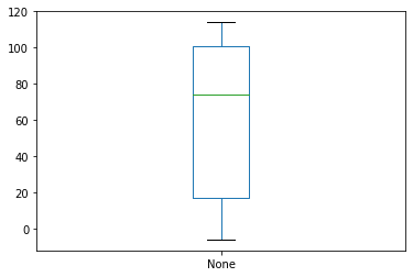
As a final flourish, and to set the scene for the next session, let’s create a boxplot showing the distribution of the time differences we calculated above.

We’ve already been introduced to so many helpful DataFrame methods (and there are many more we haven’t even mentioned) but there’s one more it’s well worth talking about here: plot.

The plot method takes an argument, kind, which specifies the type of plot we want to create from our data. A boxplot is a good choice to get a visual overview of the distribution of values among our time intervals. Unfortunately, when we try to do this Python raises another TypeError, telling us that there is “no numeric data to plot”. Apparently, pandas’ powers don’t extend to being able to plot datetime values.

We’re going to have to extract the number of days as an integer for each value in the intervals series. There’s no specific method for this operation, so we’ll have to write our own function that will access the days attribute of each datetime value, which we can then apply to the series:

def get_days(t):
    return t.days

intervals.apply(get_days).plot(kind='box')

This ability to quickly create visualisations of data stored in or generated from a dataframe or series isn’t limited to boxplots. Below are a couple more examples of the kind of figure we can produce with a call to the plot method.

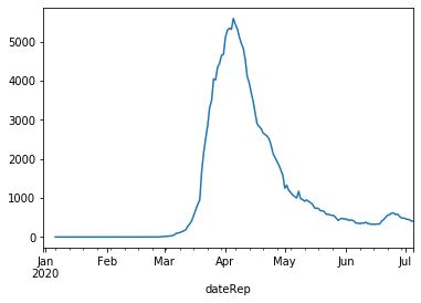
# plot rolling average for Germany
combined[combined['countriesAndTerritories']=='Germany'].set_index('dateRep')['rolling mean'].plot(kind='line')

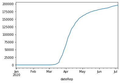
# plot cumulative sum of cases for Germany
combined[combined['countriesAndTerritories']=='Germany'].set_index('dateRep')['cases'].cumsum().plot(kind='line')

Key Points

Specialised third-party libraries such as NumPy and pandas provide powerful objects and functions that can help us analyse our data.

pandas dataframe objects allow us to efficiently load and handle large tabular data.

Use the pandas.read_csv function and DataFrame.to_csv method to read and write tabular data.

previous episode

Intermediate Python

next episode

Working with Data

Overview

NumPy

What Data to Use with NumPy?

Reading Data to a NumPy Array

The Basic Features of NumPy Arrays

2.1. Exploring Image Arrays

Solution

Indexing Arrays

2.2. Subsetting a NumPy Array

Solution

Boolean Indexing

2.3. Masking Arrays

Solution

The Power of Vectorisation

NumPy Data Types

2.4. Working with Data Types

Solution

pandas

Loading Data

Jupyter 🧡 pandas

Working with Dataframes

Selecting Data in a Dataframe

DataFrame ≠ ndarray

Filtering Data in a Dataframe

2.5. What’s going on?

Solution

Accidentally Omitted Data

Advanced Filtering

2.6. Filtering Practice

Solution

2.7. Working with Filtered Data

Solution

Combining Dataframes

2.8. Concatenating Dataframes

Solution

2.9. Working with an Indexed Dataframe

Solution

Working with Datetime Columns

2.10. Practice with Datetime Conversions

Solution

2.11. Joined in Hole-y Partnership

Solution

Further Reading - Combining Series & Dataframes

Groupby & Split-Apply-Combine

Step 1: If I Could Turn Back Time

2. Like a Complete Unknown

2.12. Writing Data to File

Solution

3. Rolling It Together

4. How Long Has It Been?

2.13. Conquering the Peaks

Solution

5. In The Middle

Conclusion

Post-Credits Bonus - Plotting with pandas

Key Points

previous episode

next episode

`DataFrame` ≠ `ndarray`