Starting with data
Data Carpentry contributors
Learning Objectives
- Load external data from a .csv file into a data frame.
- Describe what a data frame is.
- Summarize the contents of a data frame.
- Use indexing to subset specific portions of data frames.
- Describe what a factor is.
- Convert between strings and factors.
- Reorder and rename factors.
- Change how character strings are handled in a data frame.
- Format dates.
Presentation of the Survey Data
We are studying the species repartition and weight of animals caught in plots in our study area. The dataset is stored as a comma separated value (CSV) file. Each row holds information for a single animal, and the columns represent:
| Column | Description |
|---|---|
| record_id | Unique id for the observation |
| month | month of observation |
| day | day of observation |
| year | year of observation |
| plot_id | ID of a particular plot |
| species_id | 2-letter code |
| sex | sex of animal (“M”, “F”) |
| hindfoot_length | length of the hindfoot in mm |
| weight | weight of the animal in grams |
| genus | genus of animal |
| species | species of animal |
| taxon | e.g. Rodent, Reptile, Bird, Rabbit |
| plot_type | type of plot |
We are going to use the R function download.file() to
download the CSV file that contains the survey data from Figshare, and
we will use read.csv() to load into memory the content of
the CSV file as an object of class data.frame. Inside the
download.file command, the first entry is a character string with the
source URL (“https://ndownloader.figshare.com/files/2292169”). This
source URL downloads a CSV file from figshare. The text after the comma
(“data_raw/portal_data_joined.csv”) is the destination of the file on
your local machine. You’ll need to have a folder on your machine called
“data_raw” where you’ll download the file. So this command downloads a
file from Figshare, names it “portal_data_joined.csv” and adds it to a
preexisting folder named “data_raw”.
download.file(url = "https://ndownloader.figshare.com/files/2292169",
              destfile = "data_raw/portal_data_joined.csv")
You can put the arguments to a function on different lines. As long as they are within the round parentheses and each line ends with a comma, R will understand. (As above)
You are now ready to load the data:
surveys <- read.csv("data_raw/portal_data_joined.csv",
                    stringsAsFactors = TRUE)
This statement doesn’t produce any output because, as you might recall, assignments don’t display anything.
We have used the argument stringsAsFactors = TRUE here.
We will explain why in the ‘factors’ section below.
If we want to check that our data has been loaded, we can see the
contents of the data frame by typing its name: surveys.
Wow… that was a lot of output. At least it means the data loaded
properly. Let’s check the top (the first 6 lines) of this data frame
using the function head():
head(surveys)#> record_id month day year plot_id species_id sex hindfoot_length weight
#> 1 1 7 16 1977 2 NL M 32 NA
#> 2 72 8 19 1977 2 NL M 31 NA
#> 3 224 9 13 1977 2 NL NA NA
#> 4 266 10 16 1977 2 NL NA NA
#> 5 349 11 12 1977 2 NL NA NA
#> 6 363 11 12 1977 2 NL NA NA
#> genus species taxa plot_type
#> 1 Neotoma albigula Rodent Control
#> 2 Neotoma albigula Rodent Control
#> 3 Neotoma albigula Rodent Control
#> 4 Neotoma albigula Rodent Control
#> 5 Neotoma albigula Rodent Control
#> 6 Neotoma albigula Rodent Control## Try also
View(surveys)Note
read.csvassumes that fields are delineated by commas, however, in several countries, the comma is used as a decimal separator and the semicolon (;) is used as a field delineator. If you want to read in this type of files in R, you can use theread.csv2function. It behaves exactly likeread.csvbut uses different parameters for the decimal and the field separators. If you are working with another format, they can be both specified by the user. Check out the help forread.csv()by typing?read.csvto learn more. There is also theread.delim()for in tab separated data files. It is important to note that all of these functions are actually wrapper functions for the mainread.table()function with different arguments. As such, the surveys data above could have also been loaded by usingread.table()with the separation argument as,. The code is as follows:surveys <- read.table(file="data_raw/portal_data_joined.csv", sep=",", header=TRUE). The header argument has to be set to TRUE to be able to read the headers as by defaultread.table()has the header argument set to FALSE.In addition to the above versions of the csv format, you should develop the habits of looking at and record some parameters of your csv files. For instance, the character encoding, control characters used for line ending, date format (if the date is not splitted into three variables), and the presence of unexpected newlines are important characteristics of your data files. Those parameters will ease up the import step of your data in R.
What are data frames?
Data frames are the de facto data structure for most tabular data, and what we use for statistics and plotting.
A data frame can be created by hand, but most commonly they are
generated by the functions read.csv() or
read.table(); in other words, when importing spreadsheets
from your hard drive (or the web).
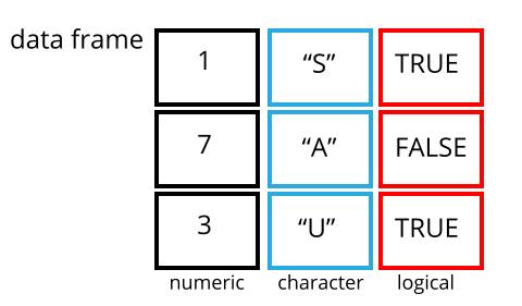
A data frame is the representation of data in the format of a table where the columns are vectors that all have the same length. Because columns are vectors, each column must contain a single type of data (e.g., characters, integers, factors). For example, here is a figure depicting a data frame comprising a numeric, a character, and a logical vector.
We can see this when inspecting the structure of a data frame
with the function str():
str(surveys)Inspecting data.frame Objects
We already saw how the functions head() and
str() can be useful to check the content and the structure
of a data frame. Here is a non-exhaustive list of functions to get a
sense of the content/structure of the data. Let’s try them out!
- Size:
dim(surveys)- returns a vector with the number of rows in the first element, and the number of columns as the second element (the dimensions of the object)nrow(surveys)- returns the number of rowsncol(surveys)- returns the number of columns
- Content:
head(surveys)- shows the first 6 rowstail(surveys)- shows the last 6 rows
- Names:
names(surveys)- returns the column names (synonym ofcolnames()fordata.frameobjects)rownames(surveys)- returns the row names
- Summary:
str(surveys)- structure of the object and information about the class, length and content of each columnsummary(surveys)- summary statistics for each column
Note: most of these functions are “generic”, they can be used on
other types of objects besides data.frame.
Challenge
2.1 Based on the output of
str(surveys), can you answer the following questions?
- What is the class of the object
surveys?- How many rows and how many columns are in this object?
- How many species have been recorded during these surveys?
Answer
str(surveys)#> 'data.frame': 34786 obs. of 13 variables: #> $ record_id : int 1 72 224 266 349 363 435 506 588 661 ... #> $ month : int 7 8 9 10 11 11 12 1 2 3 ... #> $ day : int 16 19 13 16 12 12 10 8 18 11 ... #> $ year : int 1977 1977 1977 1977 1977 1977 1977 1978 1978 1978 ... #> $ plot_id : int 2 2 2 2 2 2 2 2 2 2 ... #> $ species_id : Factor w/ 48 levels "AB","AH","AS",..: 16 16 16 16 16 16 16 16 16 16 ... #> $ sex : Factor w/ 3 levels "","F","M": 3 3 1 1 1 1 1 1 3 1 ... #> $ hindfoot_length: int 32 31 NA NA NA NA NA NA NA NA ... #> $ weight : int NA NA NA NA NA NA NA NA 218 NA ... #> $ genus : Factor w/ 26 levels "Ammodramus","Ammospermophilus",..: 13 13 13 13 13 13 13 13 13 13 ... #> $ species : Factor w/ 40 levels "albigula","audubonii",..: 1 1 1 1 1 1 1 1 1 1 ... #> $ taxa : Factor w/ 4 levels "Bird","Rabbit",..: 4 4 4 4 4 4 4 4 4 4 ... #> $ plot_type : Factor w/ 5 levels "Control","Long-term Krat Exclosure",..: 1 1 1 1 1 1 1 1 1 1 ...## * class: data frame ## * how many rows: 34786, how many columns: 13 ## * how many species: 40 (the text "Factor w/ 40 levels" from str() tells us this. More on factors soon.
Time for a git commit
Indexing and subsetting data frames
Our survey data frame has rows and columns (it has 2 dimensions), if we want to extract some specific data from it, we need to specify the “coordinates” we want from it. Row numbers come first, followed by column numbers. However, note that different ways of specifying these coordinates lead to results with different classes.
# indices in a data.frame are [rows, columns] or [columns]
# first element in the first column of the data frame (as a vector)
surveys[1, 1]
# first element in the 6th column (as a vector)
surveys[1, 6]
# first column of the data frame (as a vector)
surveys[, 1]
# first column of the data frame (as a data.frame)
surveys[1]
# first three elements in the 7th column (as a vector)
surveys[1:3, 7]
# the 3rd row of the data frame (as a data.frame)
surveys[3, ]
# equivalent to head_surveys <- head(surveys)
head_surveys <- surveys[1:6, ]
: is a special function that creates numeric vectors of
integers in increasing or decreasing order, test 1:10 and
10:1 for instance.
You can also exclude certain indices of a data frame using the
“-” sign:
surveys[, -1]          # The whole data frame, except the first column
surveys[-c(7:34786), ] # Equivalent to head(surveys)
Data frames can be subset by calling indices (as shown previously), but also by calling their column names directly:
surveys["species_id"]       # Result is a data.frame
surveys[, "species_id"]     # Result is a vector
surveys[["species_id"]]     # Result is a vector
surveys$species_id          # Result is a vector
In RStudio, you can use the autocompletion feature to get the full and correct names of the columns. Try typing “surveys$” then pause for RStudio to show you the column names (you may need to press the ‘tab’ key). (Sometimes this doesn’t work or is slow if R is busy.)
Challenge
2.2 Create a
data.frame(surveys_200) containing only the data in row 200 of thesurveysdataset.2.3 Notice how
nrow()gave you the number of rows in adata.frame?* Use that number to pull out just the last row in the data frame. * Compare that with what you see as the last row using `tail()` to make sure it's meeting expectations. * Pull out that last row using `nrow()` instead of the row number. * Create a new data frame (`surveys_last`) from that last row.2.4 Use
nrow()to extract the row that is in the middle of the data frame. Store the content of this row in an object namedsurveys_middle.2.5 Combine
nrow()with the-notation above to reproduce the behavior ofhead(surveys), keeping just the first through 6th rows of the surveys dataset.Answer
##
surveys_200 <- surveys[200, ]
##
# Saving `n_rows` to improve readability and reduce duplication
n_rows <- nrow(surveys)
surveys_last <- surveys[n_rows, ]
tail(surveys)
surveys[nrow(surveys), ]
surveys_last <- surveys[nrow(surveys), ]
##
surveys_middle <- surveys[round(n_rows / 2), ]
##
surveys_head <- surveys[-(7:n_rows), ]
Time for a git commit
Factors
When we did str(surveys) we saw that several of the
columns consist of integers. The columns genus,
species, sex, plot_type, …
however, are of a special class called factor. Factors are
very useful and actually contribute to making R particularly well suited
to working with data. So we are going to spend a little time introducing
them.
Factors represent categorical data. They are stored as integers associated with labels and they can be ordered or unordered. While factors look (and often behave) like character vectors, they are actually treated as integer vectors by R. So you need to be very careful when treating them as strings (a “string” is a series of characters, like a word or a phrase).
Once created, factors can only contain a pre-defined set of values, known as levels. By default, R always sorts levels in alphabetical order. For instance, if you have a factor with 2 levels:
sex <- factor(c("male", "female", "female", "male"))R will assign 1 to the level "female" and
2 to the level "male" (because f
comes before m, even though the first element in this
vector is "male"). You can see this by using the function
levels() and you can find the number of levels using
nlevels():
levels(sex)
nlevels(sex)
Sometimes, the order of the factors does not matter, other times you
might want to specify the order because it is meaningful (e.g., “low”,
“medium”, “high”), it improves your visualization, or it is required by
a particular type of analysis. Here, one way to reorder our levels in
the sex vector would be:
sex # current order#> [1] male female female male
#> Levels: female malesex <- factor(sex, levels = c("male", "female"))
sex # after re-ordering#> [1] male female female male
#> Levels: male femaleIn R’s memory, these factors are represented by integers (1, 2, 3),
but are more informative than integers because factors are self
describing: "female", "male" is more
descriptive than 1, 2. Which one is “male”?
You wouldn’t be able to tell just from the integer data. Factors, on the
other hand, have this information built in. It is particularly helpful
when there are many levels (like the species names in our example
dataset).
Converting factors
If you need to convert a factor to a character vector, you use
as.character(x).
as.character(sex)In some cases, you may have to convert factors where the levels
appear as numbers (such as concentration levels or years) to a numeric
vector. For instance, in one part of your analysis the years might need
to be encoded as factors (e.g., comparing average weights across years)
but in another part of your analysis they may need to be stored as
numeric values (e.g., doing math operations on the years). This
conversion from factor to numeric is a little trickier. The
as.numeric() function returns the index values of the
factor, not its levels, so it will result in an entirely new (and
unwanted in this case) set of numbers. One method to avoid this is to
convert factors to characters, and then to numbers.
Another method is to use the levels() function.
Compare:
year_fct <- factor(c(1990, 1983, 1977, 1998, 1990))
as.numeric(year_fct)               # Wrong! And there is no warning...
as.numeric(as.character(year_fct)) # Works
as.numeric(as.vector(year_fct)) # Also works.
# as.vector() changes the factor to a vector of character objects.
# It uses character objects (instead of e.g. numerics) since these
# are the lowest common denominator for atomic data types so conversion
# is safe and won't lose any data.
Renaming factors
When your data is stored as a factor, you can use the
plot() function to get a quick glance at the number of
observations represented by each factor level. Let’s look at the number
of males and females captured over the course of the experiment:
## bar plot of the number of females and males captured during the experiment:
plot(surveys$sex)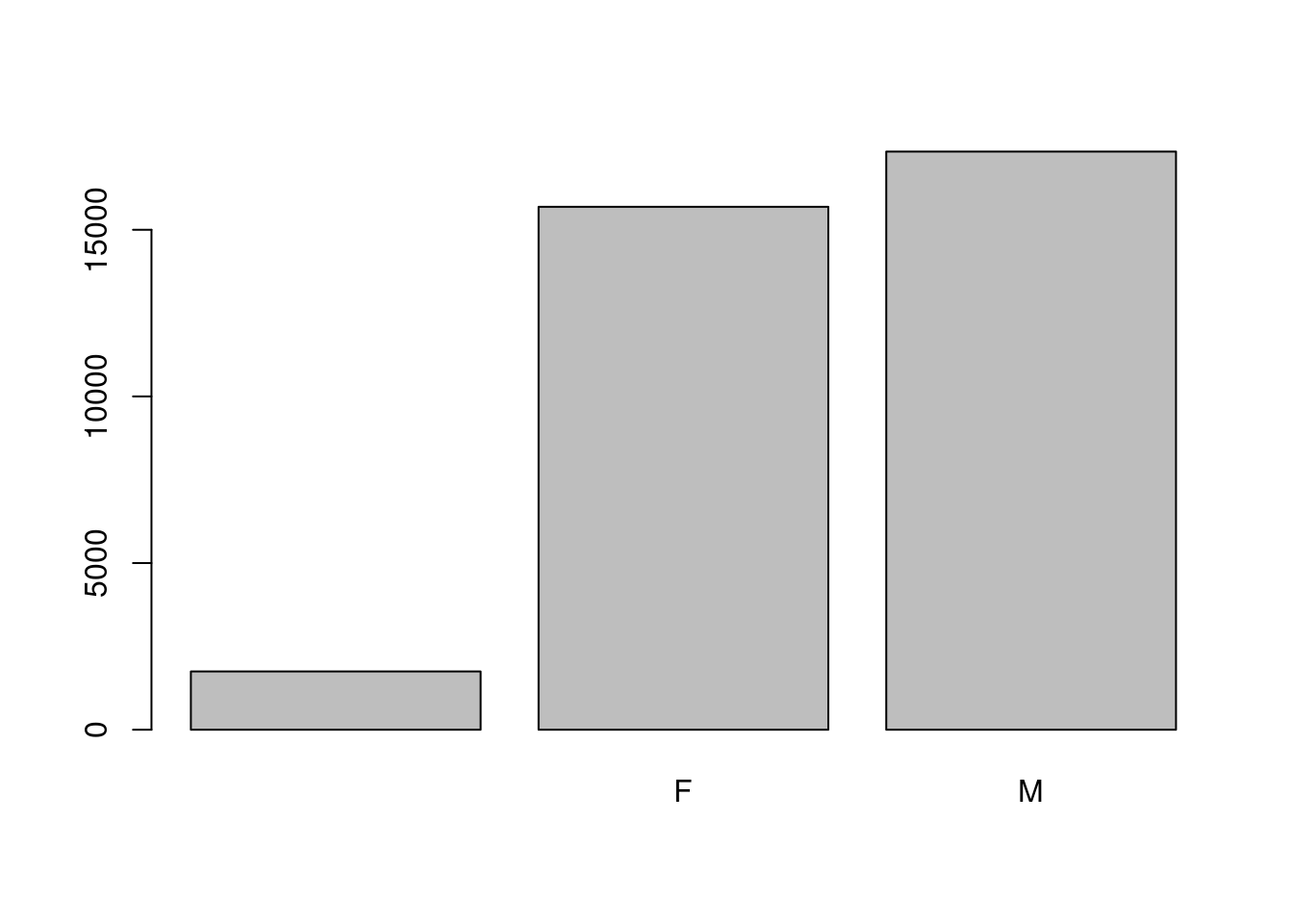
In addition to males and females, there are about 1700 individuals for which the sex information hasn’t been recorded. Additionally, for these individuals, there is no label to indicate that the information is missing or undetermined. Let’s rename this label to something more meaningful. Before doing that, we’re going to pull out the data on sex and work with that data, so we’re not modifying the working copy of the data frame:
sex <- surveys$sex
head(sex)
#> [1] M M
#> Levels: F Mlevels(sex)#> [1] "" "F" "M"levels(sex)[1] <- "undetermined"
levels(sex)#> [1] "undetermined" "F" "M"head(sex)#> [1] M M undetermined undetermined undetermined
#> [6] undetermined
#> Levels: undetermined F MChallenge
- 2.6 Rename “F” and “M” to “female” and “male” respectively.
- 2.7 Now that we have renamed the factor level to “undetermined”, can you recreate the barplot such that “undetermined” is last (after “male”)?
Answer
levels(sex)[2:3] <- c("female", "male")
sex <- factor(sex, levels = c("female", "male", "undetermined"))
plot(sex)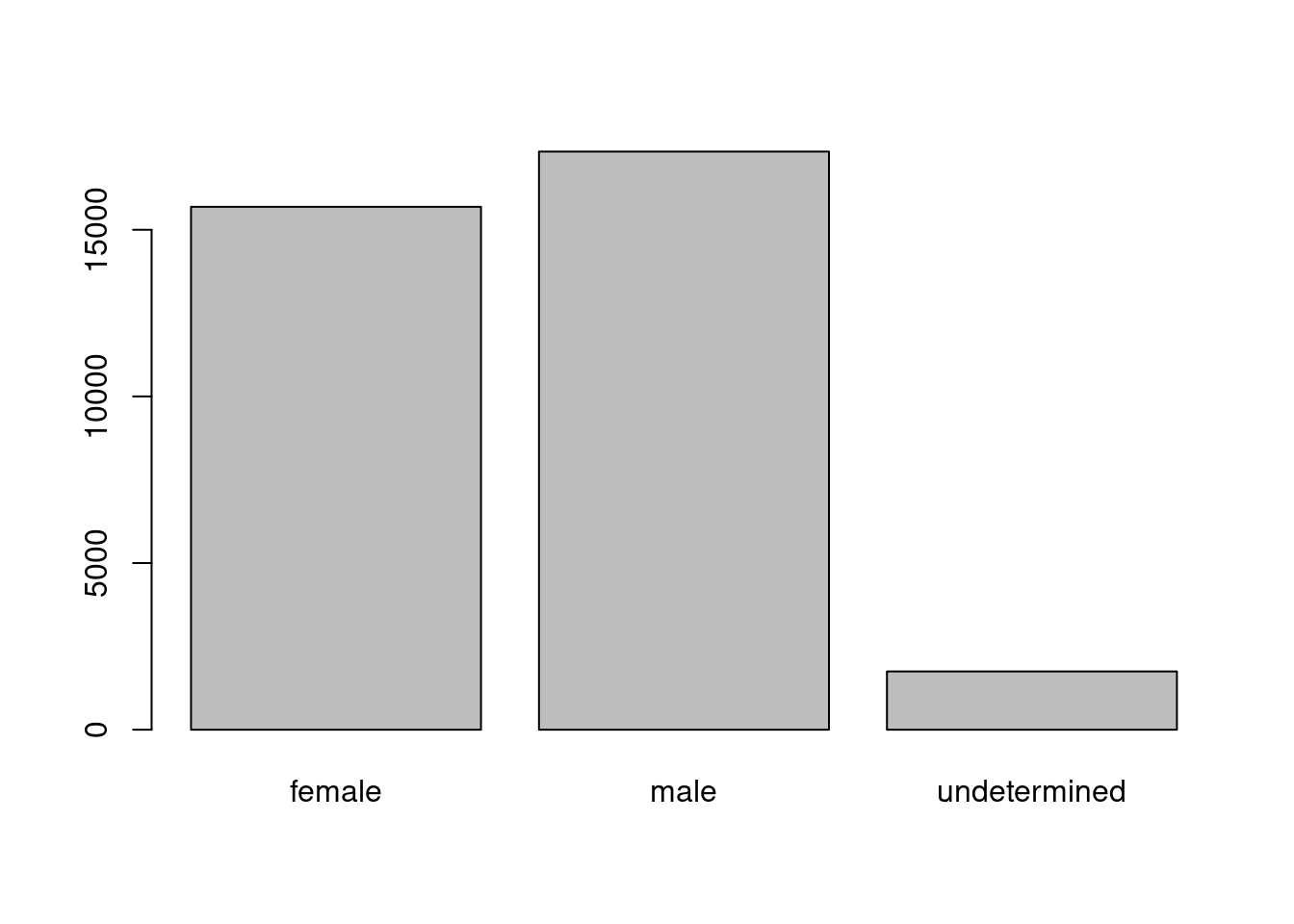
Using stringsAsFactors=FALSE
In the read.csv command at the begining of this section,
we used the argument stringsAsFactors=TRUE. This means that
when building/importing the data frame, the columns that contain
characters (i.e. text) are coerced (= converted) into factors.
Depending on what you want to do with the data, you may want to keep
these columns as character. To do so,
read.csv() and read.table() you can set
stringsAsFactors to FALSE.
In most cases, it is preferable to set
stringsAsFactors = FALSE when importing data and to convert
as a factor only the columns that require this data type.
On 2020-04-24, version 4 of R was released. Some of you have version
4 and some of you probably have version 3. (Try running
sessionInfo() to see which you have). The only difference
between these versions that matters to us is that the default value of
stringsAsFactors has been changed from TRUE in
v3 to FALSE in v4. Changing the default behaviour of a
function is rare but can occur. For this reason, it is good practice to
print out the versions of R and all your packages by calling
sessionInfo(). This way your code will be reproducible. In
the case of stringsAsFactors, since it is a recent change,
it is a good idea to be explicit about this argument value in your
code.
## Compare the difference between our data read as `factor` vs `character`.
surveys <- read.csv("data_raw/portal_data_joined.csv", stringsAsFactors = TRUE)
str(surveys)
surveys <- read.csv("data_raw/portal_data_joined.csv", stringsAsFactors = FALSE)
str(surveys)
## Convert the column "plot_type" into a factor
surveys$plot_type <- factor(surveys$plot_type)
Challenge
2.8 We have seen how data frames are created when using
read.csv(), but they can also be created by hand with thedata.frame()function. There are a few mistakes in this hand-crafteddata.frame. Can you spot and fix them? Don’t hesitate to experiment!animal_data <- data.frame( animal = c(dog, cat, sea cucumber, sea urchin), feel = c("furry", "squishy", "spiny"), weight = c(45, 8 1.1, 0.8) )2.9 Can you predict the class for each of the columns in the following example? Check your guesses using
str(country_climate):
Are they what you expected? Why? Why not?
What would have been different if we had added
stringsAsFactors = FALSEwhen creating the data frame?Can you gues the best data type for each column? What would you need to change to ensure that each column had the most appropriate data types?
country_climate <- data.frame(
       country = c("Canada", "Panama", "South Africa", "Australia"),
       climate = c("cold", "hot", "temperate", "hot/temperate"),
       temperature = c(10, 30, 18, "15"),
       northern_hemisphere = c(TRUE, TRUE, FALSE, "FALSE"),
       has_kangaroo = c(FALSE, FALSE, FALSE, 1)
       )
Answer
Data frame 1 errors: * missing quotations around the names of the animals * missing one entry in the
feelcolumn (probably for one of the furry animals) * missing one comma in theweightcolumn (between 8 and 1.1) # *country,climate,temperature, andnorthern_hemisphereare factors;has_kangaroois numeric * usingstringsAsFactors = FALSEwould have made character vectors instead of factors * removing the quotes intemperatureandnorthern_hemisphereand replacing 1 by TRUE in thehas_kangaroocolumn would give what was probably intended
The automatic conversion of data type is sometimes a blessing, sometimes an annoyance. Be aware that it exists, learn the rules, and double check that data you import in R are of the correct type within your data frame. If not, use it to your advantage to detect mistakes that might have been introduced during data entry (for instance, a letter in a column that should only contain numbers).
After the workshop, you can learn more in this RStudio tutorial
Time for a git commit
Formatting Dates
One of the most common issues that new (and experienced!) R users have is converting date and time information into a variable that is appropriate and usable during analyses.
Often the best way to handle dates is by storing each component of your date (i.e. day, month, year) as a separate variable. This means that dates like ‘01/03/02’ will never be misinterpreted (January 3 2002? March 2 2001?) and Excel won’t create problems by incorrectly converting your dates.
Using str(), we can confirm that our data frame has a
separate column for day, month, and year, and that each contains integer
values.
str(surveys)We are going to use the ymd() function from the package
lubridate.
“Packages” in R are sets of functions written by other R users that let you do more stuff more easily. There are packages made to handle different biological data types (e.g. RNASeq data, microbiome data), do fancy plotting tasks, run machine learning, etc. etc. The functions we’ve been using so far, like str() or data.frame(), come built into R. Loading additional packages gives you access to more functions.
Before you use a package for the first time you need to install it on your machine, and then you should import it in every subsequent R session when you need it. It’s a good idea to do this at the top of your R script.
Advanced discussion: lubridate belongs to the
tidyverse; learn more here). lubridate gets
installed as part as the tidyverse installation. When you
load the tidyverse (library(tidyverse)), the
core packages (the packages used in most data analyses) get loaded.
lubridate however does not belong to the core tidyverse, so
you have to load it explicitly with library(lubridate)
Start by loading the required package:
# you already installed this package when you installed the package called 'tidyverse'
library(lubridate)
ymd() takes a vector representing year, month, and day,
and converts it to a Date vector. Date is a
class of data recognized by R as being a date and can be manipulated as
such. The argument that the function requires is flexible, but, as a
best practice, is a character vector formatted as “YYYY-MM-DD”.
Let’s create a date object and inspect the structure:
my_date <- ymd("2015-01-01")
str(my_date)
We can use the paste() function to combine character
objects into one character object. The sep argument allows
you to specify what to put between the character objects.
# sep indicates the character(s) to use to separate each component
paste("2015", "1", "1", sep = "-")
Now let’s use paste() to combine the year, month, and day. We get the same result:
my_date <- ymd(paste("2015", "1", "1", sep = "-"))
str(my_date)
Now we apply this function to the surveys dataset. The
paste() function can also take vectors and will combine the
first element from each vector into one character object, then do the
second element of each vector, etc. Run this example:
letters_lower <- c("a","b","c")
letters_upper <- c("A","B","C")
paste(letters_lower , letters_upper, sep="_")
Now we can create a character vector from the year,
month, and day columns of surveys
using paste():
paste(surveys$year, surveys$month, surveys$day, sep = "-")This character vector can be used as the argument for
ymd():
ymd(paste(surveys$year, surveys$month, surveys$day, sep = "-"))#> Warning: 129 failed to parse.The resulting Date vector can be added to
surveys as a new column called date:
surveys$date <- ymd(paste(surveys$year, surveys$month, surveys$day, sep = "-"))#> Warning: 129 failed to parse.You may have gotten a warning here. Let’s make sure everything worked
correctly. One way to inspect the new column is to use
summary():
str(surveys) # notice the new column, with 'date' as the class#> 'data.frame': 34786 obs. of 14 variables:
#> $ record_id : int 1 72 224 266 349 363 435 506 588 661 ...
#> $ month : int 7 8 9 10 11 11 12 1 2 3 ...
#> $ day : int 16 19 13 16 12 12 10 8 18 11 ...
#> $ year : int 1977 1977 1977 1977 1977 1977 1977 1978 1978 1978 ...
#> $ plot_id : int 2 2 2 2 2 2 2 2 2 2 ...
#> $ species_id : Factor w/ 48 levels "AB","AH","AS",..: 16 16 16 16 16 16 16 16 16 16 ...
#> $ sex : Factor w/ 3 levels "","F","M": 3 3 1 1 1 1 1 1 3 1 ...
#> $ hindfoot_length: int 32 31 NA NA NA NA NA NA NA NA ...
#> $ weight : int NA NA NA NA NA NA NA NA 218 NA ...
#> $ genus : Factor w/ 26 levels "Ammodramus","Ammospermophilus",..: 13 13 13 13 13 13 13 13 13 13 ...
#> $ species : Factor w/ 40 levels "albigula","audubonii",..: 1 1 1 1 1 1 1 1 1 1 ...
#> $ taxa : Factor w/ 4 levels "Bird","Rabbit",..: 4 4 4 4 4 4 4 4 4 4 ...
#> $ plot_type : Factor w/ 5 levels "Control","Long-term Krat Exclosure",..: 1 1 1 1 1 1 1 1 1 1 ...
#> $ date : Date, format: "1977-07-16" "1977-08-19" ...summary(surveys$date)#> Min. 1st Qu. Median Mean 3rd Qu. Max.
#> "1977-07-16" "1984-03-12" "1990-07-22" "1990-12-15" "1997-07-29" "2002-12-31"
#> NA's
#> "129"See the NA’s? This means something went wrong: some dates have missing values. Let’s investigate where they are coming from.
We can use the functions we saw previously to deal with missing data
to identify the rows in our data frame that are failing. If we combine
them with what we learned about subsetting data frames earlier, we can
extract the columns “year,”month”, “day” from the records that have
NA in our new column date. We will also use
head() so we don’t clutter the output:
# get the rows where date is NA and the columns called year, month, and day
missing_dates <- surveys[is.na(surveys$date), c("year", "month", "day")]
# show the first 6 rows
head(missing_dates)
#> year month day
#> 3144 2000 9 31
#> 3817 2000 4 31
#> 3818 2000 4 31
#> 3819 2000 4 31
#> 3820 2000 4 31
#> 3856 2000 9 31Why did these dates fail to parse? If you had to use these data for your analyses, how would you deal with this situation?
Hint: Which months have 31 days?
Time for a git commit
Summary of functions in this lesson
download.file()# download files from the internet to your computerread.csv()# load CSV file into R memory (be careful withstringsAsFactors)head()# shows the first 6 rowsView()# invoke a spreadsheet-style data viewerread.table()# load a file in table format into R memory (be careful withstringsAsFactors)str()# check structure of the object and information about the class, length and content of each columndim()# check dimension of data framenrow()# returns the number of rowsncol()# returns the number of columnstail()# shows the last 6 rows of a dataframe or elements in a vectorcolnames()# returns the column names of a dataframe (synonym of names() for data frame objects)rownames()# returns the row names of a dataframesummary()# summary statistics for a vector or each column in a dataframefactor()# create factorslevels()# check levels of a factornlevels()# get number of levels of a factoras.character()# convert an object to a character vectoras.numeric()# convert an object to a numeric vectoras.numeric(as.character(x))# convert factors where the levels appear as characters to a numeric vectordata.frame()# create a data.frame objectymd()# convert a vector representing year, month, and day to a Date vectorpaste()# convert arguments to character objects and stick them together (concatenate)
Page built on: 📆 2023-04-18 ‒ 🕢 13:20:14
Data Carpentry, 2014-2019.
Questions? Feedback?
Please file
an issue on GitHub.
On Twitter: @datacarpentry
If this lesson is useful to you, consider